Monte Carlo and Root Finding¶

The Monty-Hall Game¶

%%html
<iframe width="800" height="450" src="https://www.youtube.com/embed/rn1y-HrmA5c?end=23" frameborder="0" allow="accelerometer; autoplay; clipboard-write; encrypted-media; gyroscope; picture-in-picture" allowfullscreen></iframe>

Is it better to change the initial pick? What is the chance of winning if we change?

Hint: There are two doors to choose from, and only one of the doors has treasure behind.

Let’s use the following program to play the game a couple of times.

import random


def play_monty_hall(num_of_doors=3):
    """Main function to run the Monty Hall game."""
    doors = {str(i) for i in range(num_of_doors)}
    door_with_treasure = random.sample(doors, 1)[0]

    # Input initial pick of the door.
    while True:
        initial_pick = input(f'Pick a door from {", ".join(sorted(doors))}: ')
        if initial_pick in doors:
            break

    # Open all but one other door. Opened door must have nothing.
    doors_to_open = doors - {initial_pick, door_with_treasure}
    other_door = (
        door_with_treasure
        if initial_pick != door_with_treasure
        else doors_to_open.pop()
    )
    print("Door(s) with nothing behind:", *doors_to_open)

    # Allow player to change the initial pick the other (unopened) door.
    change_pick = (
        input(f"Would you like to change your choice to {other_door}? [y/N] ").lower()
        == "y"
    )

    # Check and record winning.
    if not change_pick:
        mh_stats["# no change"] += 1
        if door_with_treasure == initial_pick:
            mh_stats["# win without changing"] += 1
            return print("You won!")
    else:
        mh_stats["# change"] += 1
        if door_with_treasure == other_door:
            mh_stats["# win by changing"] += 1
            return print("You won!")
    print(f"You lost. The door with treasure is {door_with_treasure}.")


mh_stats = dict.fromkeys(
    ("# win by changing", "# win without changing", "# change", "# no change"), 0
)


def monty_hall_statistics():
    """Print the statistics of the Monty Hall games."""
    print("-" * 30, "Statistics", "-" * 30)
    if mh_stats["# change"]:
        print(
            f"% win by changing: \
        {mh_stats['# win by changing'] / mh_stats['# change']:.0%}"
        )
    if mh_stats["# no change"]:
        print(
            f"% win without changing: \
        {mh_stats['# win without changing']/mh_stats['# no change']:.0%}"
        )

play_monty_hall()
monty_hall_statistics()

You may also play the game online.

To get a good estimate of the chance of winning, we need to play the game many times.
We can write a Monty-Carlo simulation instead.

# Do not change any variables defined here, or some of the tests may fail.
import numpy as np

np.random.randint?

np.random.seed(0)  # for reproducible result
num_of_games = int(10e7)
door_with_treasure = np.random.randint(1, 4, num_of_games, dtype=np.uint8)
initial_pick = np.random.randint(1, 4, num_of_games, dtype=np.uint8)

print(f"{'Door with treasure:':>19}", *door_with_treasure[:10], "...")
print(f"{'Initial pick:':>19}", *initial_pick[:10], "...")

Door with treasure: 1 3 1 3 1 2 3 3 1 1 ...
      Initial pick: 1 2 1 2 1 1 1 1 2 2 ...

door_with_treasure stores as 8-bit unsigned integers uint8 the door numbers randomly chosen from \(\{1, 2, 3\}\) as the doors with treasure behind for a number num_of_games of Monty-Hall games.
initial_pick stores the initial choices for the different games.

If players do not change their initial pick, the chance of winning can be estimated as follows:

def estimate_chance_of_winning_without_change(door_with_treasure, initial_pick):
    """Estimate the chance of winning the Monty Hall game without changing
    the initial pick using the Monte Carlo simulation of door_with_treasure
    and initial_pick."""
    count_of_win = 0
    for x, y in zip(door_with_treasure, initial_pick):
        if x == y:
            count_of_win += 1
    return count_of_win / n


n = num_of_games // 100
estimate_chance_of_winning_without_change(door_with_treasure[:n], initial_pick[:n])

0.333291

However, the above code is inefficient and takes a long time to run. You may try running it on the entire sequences of door_with_treasure and initial_pick but DO NOT put the code in your notebook, as the server refuses to autograde notebooks that take too much time or memory to run.

A simpler and also more efficient solution with well over 100 times speed up is as follows:

def estimate_chance_of_winning_without_change(door_with_treasure, initial_pick):
    """Estimate the chance of winning the Monty Hall game without changing
    the initial pick using the Monte Carlo simulation of door_with_treasure
    and initial_pick."""
    return (door_with_treasure == initial_pick).mean()


estimate_chance_of_winning_without_change(door_with_treasure, initial_pick)

0.33332177

The code uses the method mean of ndarray that computes the mean of the numpy array.
In computing the mean, True and False are regarded as 1 and 0 respectively, as illustrated below.

for i in True, False:
    for j in True, False:
        print(f"{i} + {j} == {i + j}")

True + True == 2
True + False == 1
False + True == 1
False + False == 0

Exercise Define the function estimate_chance_of_winning_by_change same as estimate_chance_of_winning_without_change above but returns the estimate of the chance of winning by changing the initial choice instead. Again, implement efficiently or jupyterhub may refuse to autograde your entire notebook.

Hint: Since there are only two unopened doors at the end of each game, a player will win by changing the initial pick if the initially picked door is not the door with treasure behind.

def estimate_chance_of_winning_by_change(door_with_treasure, initial_pick):
    """Estimate the chance of winning the Monty Hall game by changing
    the initial pick using the Monte Carlo simulation of door_with_treasure
    and initial_pick."""
    # YOUR CODE HERE
    raise NotImplementedError()

# tests
assert np.isclose(
    estimate_chance_of_winning_by_change(door_with_treasure[:10], initial_pick[:10]),
    0.7,
)

Solving a 3-by-3 system of linear equations¶

numpy has a module linalg for linear algebra, and the module provides a function called solve that can solve a system of linear equations. For the example in the lecture

\[\begin{split} \begin{aligned} 2 x_0 + 2 x_1 &= 1\\ 2 x_1 &= 1, \end{aligned} \end{split}\]

we can obtain the solution as follows:

np.linalg.solve?
A = np.array([[2.0, 2], [0, 2]])
b = np.array([1.0, 1])
x = np.linalg.solve(A, b)

As explained in the lecture, the arguments A and b are obtained from the matrix form of the system of linear equations:

\[\begin{split} \underbrace{ \begin{bmatrix} 2 & 2\\ 0 & 2 \end{bmatrix}}_{\mathbf{A}} \underbrace{ \begin{bmatrix} x_0\\ x_1 \end{bmatrix}}_{\mathbf{x}} = \underbrace{ \begin{bmatrix} 1 \\ 1 \end{bmatrix} }_{\mathbf{b}} \end{split}\]

However, the function returns an error when there is no unique solution.

# Case with infinitely many solution
A = np.array([[2.0, 2], [2, 2]])
b = np.array([1.0, 1])
x = np.linalg.solve(A, b)

---------------------------------------------------------------------------
LinAlgError                               Traceback (most recent call last)
<ipython-input-12-35be345027e3> in <module>
      2 A = np.array([[2.0, 2], [2, 2]])
      3 b = np.array([1.0, 1])
----> 4 x = np.linalg.solve(A, b)

<__array_function__ internals> in solve(*args, **kwargs)

~/my-conda-envs/jb/lib/python3.8/site-packages/numpy/linalg/linalg.py in solve(a, b)
    391     signature = 'DD->D' if isComplexType(t) else 'dd->d'
    392     extobj = get_linalg_error_extobj(_raise_linalgerror_singular)
--> 393     r = gufunc(a, b, signature=signature, extobj=extobj)
    394 
    395     return wrap(r.astype(result_t, copy=False))

~/my-conda-envs/jb/lib/python3.8/site-packages/numpy/linalg/linalg.py in _raise_linalgerror_singular(err, flag)
     86 
     87 def _raise_linalgerror_singular(err, flag):
---> 88     raise LinAlgError("Singular matrix")
     89 
     90 def _raise_linalgerror_nonposdef(err, flag):

LinAlgError: Singular matrix

# Case without solution
A = np.array([[2.0, 2], [2, 2]])
b = np.array([1.0, 0])
x = np.linalg.solve(A, b)

---------------------------------------------------------------------------
LinAlgError                               Traceback (most recent call last)
<ipython-input-13-830bec228091> in <module>
      2 A = np.array([[2.0, 2], [2, 2]])
      3 b = np.array([1.0, 0])
----> 4 x = np.linalg.solve(A, b)

<__array_function__ internals> in solve(*args, **kwargs)

~/my-conda-envs/jb/lib/python3.8/site-packages/numpy/linalg/linalg.py in solve(a, b)
    391     signature = 'DD->D' if isComplexType(t) else 'dd->d'
    392     extobj = get_linalg_error_extobj(_raise_linalgerror_singular)
--> 393     r = gufunc(a, b, signature=signature, extobj=extobj)
    394 
    395     return wrap(r.astype(result_t, copy=False))

~/my-conda-envs/jb/lib/python3.8/site-packages/numpy/linalg/linalg.py in _raise_linalgerror_singular(err, flag)
     86 
     87 def _raise_linalgerror_singular(err, flag):
---> 88     raise LinAlgError("Singular matrix")
     89 
     90 def _raise_linalgerror_nonposdef(err, flag):

LinAlgError: Singular matrix

A unique solution does not exist if and only if the determinant of \(\mathbf{A}\) is \(0\), in which case \(\mathbf{A}\) is called a singular matrix. For a \(2\)-by-\(2\) matrix, the determinant is defined as follows:

\[\begin{split} \begin{aligned} \operatorname{det}(A) &:= \left| \begin{matrix} a_{00} & a_{01}\\ a_{10} & a_{11} \end{matrix} \right|\\ &= a_{00}\times a_{11} - a_{01}\times a_{10}. \end{aligned} \end{split}\]

For example, the first system has a unique solution because

\[\begin{split} \left| \begin{matrix} 2 & 2\\ 0 & 2 \end{matrix} \right| = 2\times 2 - 2\times 0 = 4>0. \end{split}\]

The last two systems do not have unique solutions because

\[\begin{split} \left| \begin{matrix} 2 & 2\\ 2 & 2 \end{matrix} \right| = 2\times 2 - 2\times 2 = 0. \end{split}\]

We can use the function det from np.linalg to compute the determinant as follows:

np.linalg.det?
np.linalg.det(np.array([[2.0, 2], [0, 2]])), np.linalg.det(np.array([[2.0, 2], [2, 2]]))

(4.0, 0.0)

Exercise Use the det and solve functions to assign x to the numpy array storing the solution of the following linear system if the solution is unique else None.

\[\begin{split} \begin{aligned} x_0 + 2 x_1 + 3x_2 &= 14\\ 2x_0 + x_1 + 2x_2 &= 10\\ 3 x_0 + 2x_1 + x_2 &= 10. \end{aligned} \end{split}\]

# YOUR CODE HERE
raise NotImplementedError()
x

# tests
# As the main test must be hidden, you may want to verify your solution
# as explained in the lecture using matrix multiplication.
assert isinstance(x, np.ndarray) and x.shape == (3,)

Solving non-linear equations¶

Suppose we want to solve:

\[ f(x) = 0 \]

for some possibly non-linear real-valued function \(f(x)\) in one real-valued variable \(x\). Quadratic equation with an \(x^2\) term is an example. The following is another example.

%matplotlib inline
import matplotlib.pyplot as plt
import numpy as np

f = lambda x: x * (x - 1) * (x - 2)
x = np.linspace(-0.5, 2.5)
plt.plot(x, f(x))
plt.axhline(color="gray", linestyle=":")
plt.xlabel(r"$x$")
plt.title(r"Plot of $f(x)=x(x-1)(x-2)$")
plt.show()

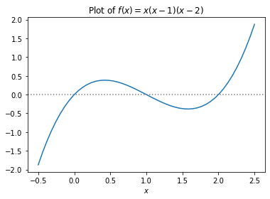
../_images/Monte Carlo and Root Finding_40_0.png

While it is clear that the above function has three roots, namely, \(x=0, 1, 2\), can we write a program to compute a root of any given continuous function \(f\)?

%%html
<iframe width="800" height="450" src="https://www.youtube.com/embed/PXSLcEGkXkU" frameborder="0" allow="accelerometer; autoplay; clipboard-write; encrypted-media; gyroscope; picture-in-picture" allowfullscreen></iframe>

The following function bisection

takes as arguments
- a continuous function f,
- two real values a and b,
- a positive integer n indicating the maximum depth of the recursion, and
returns a list [xstart, xstop] if the bisection succeeds in capturing a root in the interval [xstart, xstop] bounded by a and b, or else, returns a empty list [].

def bisection(f, a, b, n=10):
    if f(a) * f(b) > 0:
        return []  # because f(x) may not have a root between x=a and x=b
    elif n <= 0:  # base case when recursion cannot go any deeper
        return [a, b] if a <= b else [b, a]
    else:
        c = (a + b) / 2  # bisect the interval between a and b
        return bisection(f, a, c, n - 1) or bisection(f, c, b, n - 1)  # recursion


# bisection solver
import ipywidgets as widgets


@widgets.interact(a=(-0.5, 2.5, 0.5), b=(-0.5, 2.5, 0.5), n=(0, 10, 1))
def bisection_solver(a=-0.5, b=0.5, n=0):
    x = np.linspace(-0.5, 2.5)
    plt.plot(x, f(x))
    plt.axhline(color="gray", linestyle=":")
    plt.xlabel(r"$x$")
    plt.title(r"Bisection on $f(x)$")
    [xstart, xstop] = bisection(f, a, b, n)
    plt.plot([xstart, xstop], [0, 0], "r|-")
    print("Interval: ", [xstart, xstop])

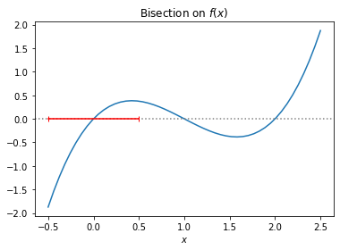
../_images/Monte Carlo and Root Finding_44_1.png

Try setting the values of \(a\) and \(b\) as follows and change \(n\) to see the change of the interval step-by-step.

bisection(f, -0.5, 0.5), bisection(f, 1.5, 0.5), bisection(f, -0.1, 2.5)

([-0.0009765625, 0.0], [1.0, 1.0009765625], [1.9998046875000002, 2.00234375])

Exercise Modify the function bisection to

take the floating point parameter tol instead of n, and
return the interval from the bisection method represented by a list [xstart,xstop] but as soon as the gap xstop - xstart is \(\leq\) tol.

def bisection(f, a, b, tol=1e-9):
    # YOUR CODE HERE
    raise NotImplementedError()

# tests
import numpy as np

f = lambda x: x * (x - 1) * (x - 2)
bisection(f, 1.5, 0.5)
assert np.isclose(bisection(f, -0.5, 0.5), [-9.313225746154785e-10, 0.0]).all()
_ = bisection(f, 1.5, 0.5, 1e-2)
assert np.isclose(_, [1.0, 1.0078125]).all() or np.isclose(_, [0.9921875, 1.0]).all()
assert np.isclose(
    bisection(f, -0.1, 2.5, 1e-3), [1.9998046875000002, 2.0004394531250003]
).all()

CS1302

Monte Carlo and Root Finding¶

The Monty-Hall Game¶

Solving a 3-by-3 system of linear equations¶

Solving non-linear equations¶