Calculators - CS1302

CS1302 Introduction to Computer Programming

Run the following to load additional tools required for this lab.
In particular, the math library provides many useful mathematical functions and constants.

import math
from math import cos, exp, log, pi, sin, tan

import jsxgraphs
import matplotlib.pyplot as plt
import numpy as np
import sympy as sp
from ipywidgets import interact

%matplotlib widget

The following code is a Python one-liner that creates a calculator.
Evaluate the cell with Ctrl+Enter:

print(eval(input()))

Try some calculations below using this calculator:

$2^3$ by entering 2**3;
$\frac23$ by entering 2/3;
$\left\lceil\frac32\right\rceil$ by entering 3//2;
$3\mod 2$ by entering 3%2;
$\sqrt{2}$ by entering 2**0.5; and
$\sin(\pi/6)$ by entering sin(pi/6);

For this lab, you will create different calculators. We will first show you a demo. Then, it will be your turn to create the calculators.

Hypotenuse Calculator¶

You can verify the theorem using the JSXGraph app below:

jsxgraphs.pythagorean1

The following is an interactive graphical proof:

jsxgraphs.pythagorean2

Another interactive proof is as follows:

jsxgraphs.pythagorean3

We can define the following function to calculate the length c of the hypotenuse when given the lengths a and b of the other sides:

def length_of_hypotenuse(a, b):
    c = (a**2 + b**2) ** (0.5)  # Pythagoras
    return c

Program 1:A function that computes the length of hypotenuse

def length_of_hypotenuse(a, b):
    # YOUR CODE HERE
    raise NotImplementedError()
    return c

You can check your code against a few cases listed in the test cell below.

# tests
assert np.isclose(length_of_hypotenuse(0, 0), 0)
assert np.isclose(length_of_hypotenuse(3, 4), 5)
assert np.isclose(length_of_hypotenuse(4, 7), 8.06225774829855)

If you are curious about the hidden test...

The hidden test will look like the following but with a "truely" random random _seed_:

rng = np.random.default_rng(_seed_)
a, b = rng.random(2)

assert np.isclose(length_of_hypotenuse(a, b), (a**2 + b**2) ** (0.5))

# hidden tests

We will use ipywidgets to let user interact with the calculator more easily as illustrated in Figure 1:

After running the cell, move the sliders to change the values of a and b.
Observer that the value of c is updated immediately.

The hypotenuse calculator — Figure 1:Illustration of the hypotenuse calculator

# hypotenuse calculator
@interact(a=(0, 10, 1), b=(0, 10, 1))
def calculate_hypotenuse(a=3, b=4):
    print('c: {:.2f}'.format(length_of_hypotenuse(a, b)))

Quadratic Equation¶

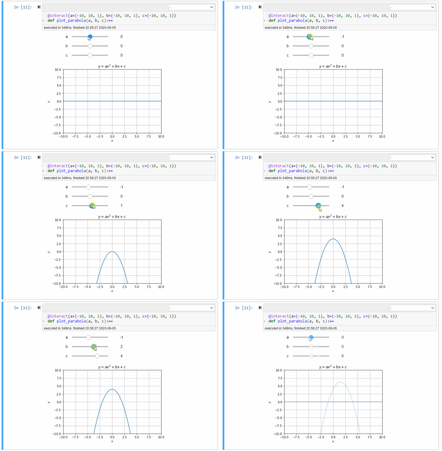
Graphical Calculator for Parabola¶

The parabola calculator — Figure 2:Illustration of the parabola calculator

The following plots the parabola with difference choices of coefficients.

jsxgraphs.parabola

def get_y(x, a, b, c):
    # YOUR CODE HERE
    raise NotImplementedError()
    return y

To test your code:

# tests
assert np.isclose(get_y(0, 0, 0, 0), 0)
assert np.isclose(get_y(0, 1, 2, 1), 1)
assert np.isclose(get_y(0, 2, 1, 2), 2)
assert np.isclose(get_y(1.2, 2, 3, 4), 10.48)
assert np.isclose(get_y(2, 3.3, 4, 5), 26.2)
assert np.isclose(get_y(3, 4.4, 5, 6), 60.6)

# hidden tests

To run the graphical calculator illustrate in Figure 2:

# graphical calculator for parabola
fig, ax = plt.subplots()
xmin, xmax, ymin, ymax, resolution = -10, 10, -10, 10, 50
x = np.linspace(xmin, xmax, resolution)
ax.set_title(r"$y=ax^2+bx+c$")
ax.set_xlabel(r"$x$")
ax.set_ylabel(r"$y$")
ax.set_xlim([xmin, xmax])
ax.set_ylim([ymin, ymax])
ax.grid()
(p,) = ax.plot(x, get_y(x, 0, 0, 0))


@interact(a=(-10, 10, 1), b=(-10, 10, 1), c=(-10, 10, 1))
def plot_parabola(a, b, c):
    p.set_ydata(get_y(x, a, b, c))

Quadratic Equation Solver¶

def get_roots(a, b, c):
    # YOUR CODE HERE
    raise NotImplementedError()
    return root1, root2

To test your code:

# tests
assert np.isclose(get_roots(1, 1, 0), (-1.0, 0.0)).all()
assert np.isclose(get_roots(1, 2, 1), (-1.0, -1.0)).all()
assert np.isclose(get_roots(2, 2, 1), (-0.5 - 0.5j, -0.5 + 0.5j)).all()

# hidden tests

To run the calculator illustrated in Figure 3:

# quadratic equations solver
@interact(a=(-10,10,1),b=(-10,10,1),c=(-10,10,1))
def quadratic_equation_solver(a=1,b=2,c=1):
    print('Roots: {}, {}'.format(*get_roots(a,b,c)))

Number Conversion¶

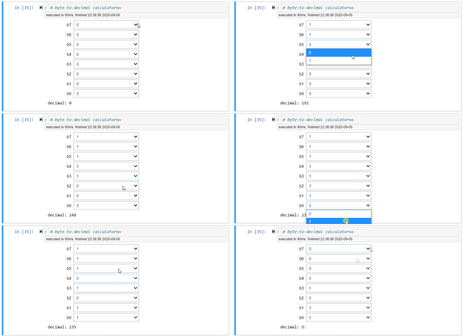
Byte-to-Decimal Calculator¶

Denote a binary number stored as a byte ( $8$ -bit) as

b_7\circ b_6\circ b_5\circ b_4\circ b_3\circ b_2\circ b_1\circ b_0,

(5)

where $\circ$ concatenates $b_i$ 's together into a binary string.

The binary string can be converted to a decimal number by the formula

b_7\cdot 2^7 + b_6\cdot 2^6 + b_5\cdot 2^5 + b_4\cdot 2^4 + b_3\cdot 2^3 + b_2\cdot 2^2 + b_1\cdot 2^1 + b_0\cdot 2^0.

(6)

E.g., the binary string '11111111' is the largest integer represented by a byte:

2^7+2^6+2^5+2^4+2^3+2^2+2^1+2^0=255=2^8-1.

(7)

def byte_to_decimal(b7, b6, b5, b4, b3, b2, b1, b0):
    """
    Parameters
    ----------
    b7, ..., b0: single characters either '0' or '1'.
    """
    # YOUR CODE HERE
    raise NotImplementedError()
    return decimal

To test your code:

# tests
def test_byte_to_decimal(decimal, b7, b6, b5, b4, b3, b2, b1, b0):
    decimal_ = byte_to_decimal(b7, b6, b5, b4, b3, b2, b1, b0)
    assert decimal == decimal_ and isinstance(decimal_, int)


test_byte_to_decimal(38, "0", "0", "1", "0", "0", "1", "1", "0")
test_byte_to_decimal(20, "0", "0", "0", "1", "0", "1", "0", "0")
test_byte_to_decimal(22, "0", "0", "0", "1", "0", "1", "1", "0")
test_byte_to_decimal(146, '1', '0', '0', '1', '0', '0', '1', '0')
test_byte_to_decimal(128, '1', '0', '0', '0', '0', '0', '0', '0')
test_byte_to_decimal(71, '0', '1', '0', '0', '0', '1', '1', '1')

# hidden tests

To run the calculator illustrate in Figure 4:

# byte-to-decimal calculator
bit = ['0', '1']


@interact(b7=bit, b6=bit, b5=bit, b4=bit, b3=bit, b2=bit, b1=bit, b0=bit)
def convert_byte_to_decimal(b7, b6, b5, b4, b3, b2, b1, b0):
    print('decimal:', byte_to_decimal(b7, b6, b5, b4, b3, b2, b1, b0))

Decimal-to-Byte Calculator¶

def decimal_to_byte(decimal):
    # YOUR CODE HERE
    raise NotImplementedError()
    return byte

To test your code:

# tests
def test_decimal_to_byte(byte, decimal):
    byte_ = decimal_to_byte(decimal)
    assert byte == byte_ and isinstance(byte, str) and len(byte) == 8


test_decimal_to_byte("01100111", 103)
test_decimal_to_byte("00000011", 3)
test_decimal_to_byte("00011100", 28)
test_decimal_to_byte('11011111', 223)
test_decimal_to_byte('00000100', 4)
test_decimal_to_byte('10011001', 153)


def test_decimal_to_byte(byte,decimal):
    byte_ = decimal_to_byte(decimal)
    correct = byte == byte_ and isinstance(byte, str) and len(byte) == 8
    if not correct:
        print(
            f'{decimal} should be represented as the byte {byte}, not {byte_}.'
        )
    assert correct


test_decimal_to_byte('01100111', 103)
test_decimal_to_byte('00000011', 3)
test_decimal_to_byte('00011100', 28)

# hidden tests

To run the calculator illustrate in Figure 5:

# decimal-to-byte calculator
@interact(decimal=(0, 255, 1))
def convert_decimal_to_byte(decimal=0):
    print("byte:", decimal_to_byte(decimal))

Symbolic calculators¶

Can we do complicated arithmetics with python. What about Calculus?

\int \tan(x)\, dx = \color{red}{?}

(8)

Try SymPy Gamma or SymPy Beta.

How does SymPy Gamma work?

SymPy Gamma is a web application running SymPy, which is a python library for symbolic computation.
SymPy Beta is a fork of SymPy Gamma that can run totally in the browser.

How to use SymPy?

The following line in the initialization cell imports the library:

import sympy as sp

We need to define a symbolic variable and assign it to a python variable.

x = sp.symbols("x")
x

The SymPy expression for $\tan(x)$ is:

f = sp.tan(x)
f

To compute the integration:

\int f(x) dx

(9)

g = sp.integrate(f)
g

To compute the derivative:

\frac{d}{dx}g(x)

(10)

diff_g = sp.diff(g)
diff_g

The answer can be simplified as expected:

diff_g.simplify()

To plot the functions:

p = sp.plot(f, g, (x, -2 * sp.pi / 5, 2 * sp.pi / 5), ylabel="y", legend=True)

# YOUR CODE HERE
raise NotImplementedError()

The following test should plot your expression f in SymPy.

# tests
assert sp.simplify(f.subs(x, 0) - 1) == 0
assert sp.simplify(f.subs(x, sp.S(1)/2) - sp.sqrt(3)*2/3) == 0

# hidden tests